I thought I'd follow up my last post with some information on some of the tools I used. I'm not going to talk about how I made the equations, because they came out terrible and I'm trying to come up with a new way. I guess if anyone is curious: I made them in LaTeX and used gimp to convert them to PNGs.
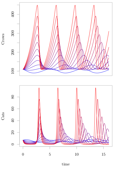
Ok, so let's see how I made the graphics. Here's the first graphic, in case anyone forgot.
The first step in creating the graphic was, obviously, to solve the ODEs. I used SciPy for that. Specifically, I used the odeint command. It's pretty simple to use in fact. Here's what it looks like:
This function is part of the NumPy python packages, so you can easily work with systems of equations, like the one seen in Predator-Prey Models and Global Warming. The function
Anyway, so that is odeint. Now, for the full script used to solve the predator-prey models:
The advantage to using SciPy is the ability to spice up the ODE with some programming, which allowed me to calculate the solution at each of the temperatures pretty easily. Now, how to graph it? I've been pretty hot on R lately for my graphs. Some people like the combination of SciPy and matplotlib, which is powerful. But, for publication quality graphics, R is what I use.
I won't go into too much detail on the script, but you can probably figure out most of it from below. The great thing about python and R is that you can open up the languages in an interactive terminal and go line by line to examine how a script works. The disadvantage to being an interactive language, especially for R, is the performance hit. Anyway, without further ado here is the R plotting script:
That's it! Now I just need to figure out how to format equations...
Ok, so let's see how I made the graphics. Here's the first graphic, in case anyone forgot.
The first step in creating the graphic was, obviously, to solve the ODEs. I used SciPy for that. Specifically, I used the odeint command. It's pretty simple to use in fact. Here's what it looks like:
This function is part of the NumPy python packages, so you can easily work with systems of equations, like the one seen in Predator-Prey Models and Global Warming. The function
derivative_fxn needs to return the derivative given x and the time. Note, that x may be an array. The args=(...) allows you to pass a tuple of arguments to give to the derivative_fxn.Anyway, so that is odeint. Now, for the full script used to solve the predator-prey models:
The advantage to using SciPy is the ability to spice up the ODE with some programming, which allowed me to calculate the solution at each of the temperatures pretty easily. Now, how to graph it? I've been pretty hot on R lately for my graphs. Some people like the combination of SciPy and matplotlib, which is powerful. But, for publication quality graphics, R is what I use.
I won't go into too much detail on the script, but you can probably figure out most of it from below. The great thing about python and R is that you can open up the languages in an interactive terminal and go line by line to examine how a script works. The disadvantage to being an interactive language, especially for R, is the performance hit. Anyway, without further ado here is the R plotting script:
That's it! Now I just need to figure out how to format equations...
