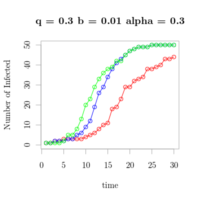
In this post, I'll describe how to go from the SIS model to a zombie model. The results are a stochastic simulation, shown below. There are few items on the model TODO list: add spatial variables and zombie deaths/kills.
I left off with the question of how to model larger populations. Matrices representing every individual will create some gnarly calculations at 100s of individuals. Really, that isn't unfeasible with a computer. I mean, in fact I could fire up my supercomputer with 1,920 CPU cores and handle at least a million. But, I think we can do better. Realistically, in order to do larger simulations with millions we'll have to move into continuous stochastic models (i.e., Brownian motion)
Previously, I tried to write as instructively as possible. Since no one ever reads what I write, I'm going to go much faster. Instead of our state vector encoding infected or susceptible, we'll have a distribution representing the number of infected. That means we only care about one number, the number of infected, though we can switch to a distribution of number healthy. The transition probabilities are:
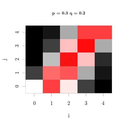
Now let's see what this equation produces. Just like last time, I'll be dealing with transition probability matrices. However, I won't be representing the matrices with numbers because they'll be too big. Instead I'll be plotting them. If we have a small population of only 4 individuals, we get this matrix:
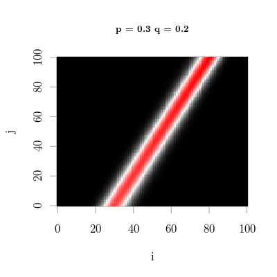
You'll notice the highest transition probabilities exist in those places with large binomial coefficients. There's a lot of interesting features in this matrix, look closely. However, I'm going to move on. Let's look at a population of 100. That is shown below:
Now we're starting to see something interesting. Notice the banding pattern, where there appears to be a constant variance to the band and there only appears to be a small number of available transitions at each step. Also, the intercepts are np and n(1 - q). My intuition is that this pattern will converge to either Brownian motion once we increase the population to infinitely sub-dividable. Let's see what happens if we change p and q.
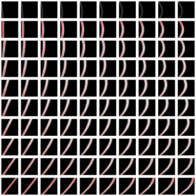
This graphic shows the transition probability matrix as a function of q and p. The top left is with probabilities of 0 for both. That means there will be no transitions, hence the solid black. The row is the value of p. For example, the bottom left has no probability of recovery and probability 1 of being infected. Hence, once you make it to all infected, you never leave. That's the tiny red dot in the upper right corner of that matrix. The diagonal of all the matrices are all doubly stochastic matrices, because p and q add up to 1. This means there is a single vertical band, in the picture at least. Doubly stochastic also means the system converges to a very simple distribution. Anyway, that image is a nice way to understand how the transition matrix changes. Notice, too, that the variance of the band seems to be related to the product of p and q. I made many graphics to describe this system, but I think that's enough for now.
Proportional SIS
Now, let's start making the model more realistic. The transition probabilities for each individual are currently constant; let's try making that more realistic. Let's assume that recovery for now is a constant probability. At least, we don't have any variables to better predict recovery. The probability of infection can be improved. We may assume that it is proportional to the number of infected. The model equation is now:
Let's take a look and see how the transition probability matrices look as a function of alpha and q. q is changing across the columns below, alpha in the rows.
It is interesting to notice how different the stochastic models look compared to deterministic models. The models head towards an equilibrium value, but they do so with some noise. I think that wraps up the SIS model for now.
SZ Model
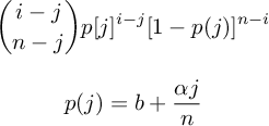
Zombies are already in our model. The rate of infection is proportional to the number of infected, just as would be expected for a finite population with zombies. The only change is that we need to remove the probability of recovery. Luckily, that simplifies the math a ton, leading to this simple equation:
The model is an easy binomial. The transition probability matrices, as a function of alpha, look like this:
Now, finally, we can see a simulation of this model and observe the differences in the time until the zombies take over.
This time the model is transient, it always reaches complete infection. Next time, we'll have to see how to add zombie deaths!
