This tutorial will show you how to reproduce the method in the recent White et al. water AIMD paper (White et al., 2017). The goal of the method is to minimally bias a water simulation to match a reference RDF. We will first convert a reference RDF into a set of reference scalar coordination number moments. Then, an NVT simulation is run to find a minimal bias which causes the coordination numbers to match their reference values. It won’t be covered here, but the bias can then be used to run NVE simulations or in conjunction with other free-energy methods. This tutorial will use classical simulations in Lammps instead of AIMD in CP2K so that results can be obtained in a reasonable amount of time.
Requirements
This tutorial utilizes Docker to run simulations and perform analysis. The only tools you’ll need are the Docker package (called docker.io on Ubuntu). Docker is available on both Windows and Linux. Git is also used for version control, but if you’d prefer not to install it you can download the tutorial files by navigating to github.com/ur-whitelab/tutorials and downloading a zip file.
Setting up
First get the Docker image to obtain required for this tutorial:
docker pull whitelab/tutorial-lammps-cn
Now let’s get the files for the tutorial. I will use [tutor-dir] to indicate the root directory which you’re using for this tutorial.
git clone https://github.com/ur-whitelab/tutorials [tutor-dir]
cd [tutor-dir]/eds-coordination-tutorial
In general, you run commands using the Docker container like this:
docker run --rm -it -v [tutor-dir]:/home/whitelab/scratch whitelab/tutorial-lammps-cn [command]
I will use pwd as a shortcut for [tutor-dir]. Note this will not
work on Windows, where you’ll need to put your complete path in
Windows path notation.
Unbiased Simulation
Let’s start by seeing what our unbiased overstructured water
simulation looks like. Our classic molecular dynamics water model
mimics the overstructuring of DFT 300K water. Begin the simulation
using this command lammps -var name unbiased -in lammps.in with the
Docker container. This runs an NVT simulation with the name
‘Unbiased’. The complete command with the docker container preamble is:
docker run --rm -it -v `pwd`:/home/whitelab/scratch whitelab/tutorial-lammps-cn lammps -var name unbiased -in lammps.in
This will take a little while and generate a few files with the label
‘unbiased’. To analyze them, we can use the included python3 script
with python3 analyze_run.py unbiased:
docker run --rm -it -v `pwd`:/home/whitelab/scratch whitelab/tutorial-lammps-cn python3 analyze_run.py unbiased
You should see a few images showing the evolution of the coordination number of water oxygen with water oxygen along with an average radial distribution function (RDF) and temperature for the simulation. Radial distribution functions (RDFs) are (transformed) probability distributions. Here’s the RDF:
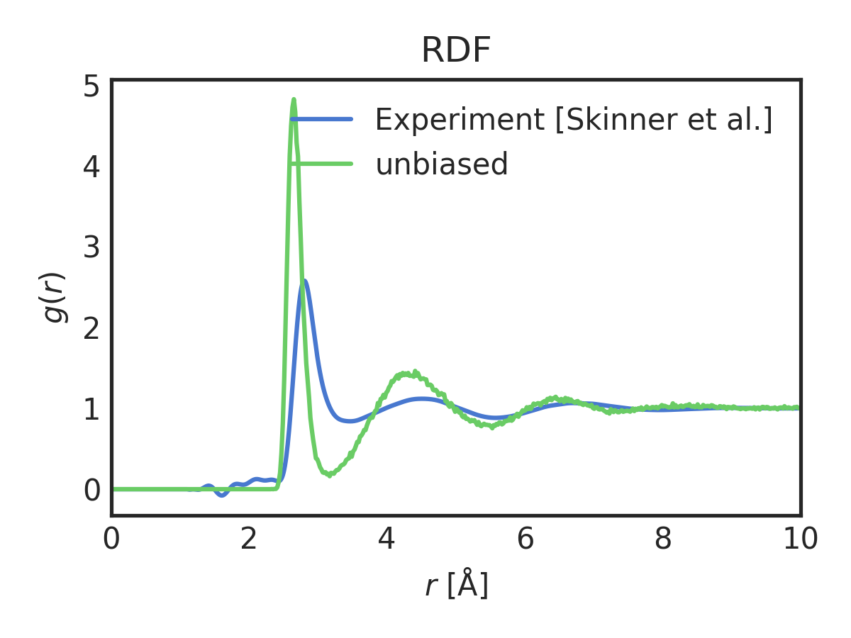
As you can see, the unbiased simulation has a significantly higher first-peak and general overstructuring relative to the experimental RDF.
Converting RDF to Coordination Number Scalars
To fix this overstructuring, we will now bias the experiment directed simulation (EDS) method (missing reference). The minimal biasing EDS method can only bias scalars (missing reference), not distributions. There is a method for minimal biasing of probability distirbutions like RDFs, but it is generally too slow to converge for use on AIMD (White et al., 2015), so we will skip it for this tutorial. Thus the first step is to convert the RDF into scalars so that EDS can be used. The implementation of EDS is in Plumed2,(Bonomi et al., 2009) which is a free-energy methods library with integration in many common simulation engines.
The chosen scalars are coordination number and moments of it. See this post for a description of the parameters involved and how to choose them. After the coordination number parameters are chosen (, , and ), the reference RDF can be used to generate the reference coordination number averages. This is done using this python this script, which is included in the tutorial files.
Let’s convert the reference RDF then into the scalar coordination numbers. This RDF is of water at 300K as determined by X-ray scattering (Skinner et al., 2013). We follow the parameters from the White et al. 2017 AIMD water paper (White et al., 2017) for the , , , , and the cutoff, but we must calculate the exact density for our system. Our simulation is 128 water molecules in a box of size 15.6629 Å. Due to how RDFs is connected to coordination number, the density is . Thus our density is 0.0333 Å .Run for each moment as shown below:
docker run --rm -it -v `pwd`:/home/whitelab/scratch whitelab/tutorial-lammps-cn python3 convert_gr.py -moment 0 -r0 2.3 -n 6 -m 12 -w 0.7 -rmax 7.0 reference.rdf aimd 0.0333

docker run --rm -it -v `pwd`:/home/whitelab/scratch whitelab/tutorial-lammps-cn python3 convert_gr.py -moment 1 -r0 2.3 -n 6 -m 12 -w 0.7 -rmax 7.0 reference.rdf aimd 0.0333

docker run --rm -it -v `pwd`:/home/whitelab/scratch whitelab/tutorial-lammps-cn python3 convert_gr.py -moment 2 -r0 2.3 -n 6 -m 12 -w 0.7 -rmax 7.0 reference.rdf aimd 0.0333

docker run --rm -it -v `pwd`:/home/whitelab/scratch whitelab/tutorial-lammps-cn python3 convert_gr.py -moment 3 -r0 2.3 -n 6 -m 12 -w 0.7 -rmax 7.0 reference.rdf aimd 0.0333
this will output the following information about the RDF:
r0 = 2.3, n = 6.0, m = 12.0, w = 0.7, Exact: 0.4297167332248187, Approximate: 2.9893015681855717
with a possible warning about the truncation error. We can run this with different values for moment to get the higher coordination number moments as well. The approximate coordination numbers are the ones we will use for biasing. For a description on the difference between the exact and approximate, see this post. The final values are
| Moment | Set-Point |
|---|---|
| 0 | 2.99 |
| 1 | 8.45 |
| 2 | 24.16 |
| 3 | 69.60 |
Note: these particular values are set in a file called
set_points.txt for generating the plots. If you experiment with
different parameters/cutoffs, be sure to change the values in the file so that
your plots correctly show them.
Biasing Water Simulation
The next step is to now bias the water simulation. We don’t need to
modify the basic simulation, but we’ll add some items to our plumed
input file. Let’s start by defining the coordination number
moments. Open the biased.plumed file and you should see:
UNITS LENGTH=A ENERGY=kcal/mol TIME=fs
oxygen: GROUP ATOMS=1-384:3
cn0: COORDINATIONNUMBER SPECIES=oxygen SWITCH={RATIONAL D_0=2.3 NN=6 MM=12 R_0=0.7 D_MAX=7 NOSTRETCH} MEAN
cn1: COORDINATIONNUMBER SPECIES=oxygen SWITCH={RATIONAL D_0=2.3 NN=6 MM=12 R_0=0.7 D_MAX=7 NOSTRETCH} R_POWER=1 MEAN
cn2: COORDINATIONNUMBER SPECIES=oxygen SWITCH={RATIONAL D_0=2.3 NN=6 MM=12 R_0=0.7 D_MAX=7 NOSTRETCH} R_POWER=2 MEAN
cn3: COORDINATIONNUMBER SPECIES=oxygen SWITCH={RATIONAL D_0=2.3 NN=6 MM=12 R_0=0.7 D_MAX=7 NOSTRETCH} R_POWER=3 MEAN
eds: EDS ARG=cn0.mean PERIOD=250 CENTER=2.99 OUT_RESTART=biased_eds.restart TEMP=300
PRINT ARG=cn0.mean,cn1.mean,cn2.mean,cn3.mean STRIDE=50 FILE=biased_cn.log
The first line sets the units to match the units in the reference
RDF. The next line creates a group for the oxygen atoms. The
parameters for the coordination number are set to match we used for
the convert_gr.py script. The R_POWER parameter is the moment,
D_MAX is the rmax (cutoff), D_0 is the w parameter and the
others are named the same. We use the NOSTRETCH keyword to ensure
our function computed on the RDF matches identically what is from
plumed. Notice as well that we use MEAN, so that we are looking at
the average coordination number moment. There is no biasing
information yet.
Now we add the biasing information. Copy the file/rename it to be
biased-1.plumed. Add the line below starts with “eds:” :
UNITS LENGTH=A ENERGY=kcal/mol TIME=fs
oxygen: GROUP ATOMS=1-384:3
cn0: COORDINATIONNUMBER SPECIES=oxygen SWITCH={RATIONAL D_0=2.3 NN=6 MM=12 R_0=0.7 D_MAX=7 NOSTRETCH} MEAN
cn1: COORDINATIONNUMBER SPECIES=oxygen SWITCH={RATIONAL D_0=2.3 NN=6 MM=12 R_0=0.7 D_MAX=7 NOSTRETCH} R_POWER=1 MEAN
cn2: COORDINATIONNUMBER SPECIES=oxygen SWITCH={RATIONAL D_0=2.3 NN=6 MM=12 R_0=0.7 D_MAX=7 NOSTRETCH} R_POWER=2 MEAN
cn3: COORDINATIONNUMBER SPECIES=oxygen SWITCH={RATIONAL D_0=2.3 NN=6 MM=12 R_0=0.7 D_MAX=7 NOSTRETCH} R_POWER=3 MEAN
eds: EDS ARG=cn0.mean PERIOD=250 CENTER=2.99 OUT_RESTART=biased_eds.restart TEMP=300
PRINT ARG=cn0.mean,cn1.mean,cn2.mean,cn3.mean STRIDE=50 FILE=biased_cn.log
We’re only biasing the coordination number (0th moment) with this
one. Remember to rename this file to be biased-1.plumed. Our period
was selected to be 250 timesteps (125 fs), which gives the simulation
sometime to adjust to changes to the bias.
Now are ready to start the simulation. Begin it with:
docker run --rm -it -v `pwd`:/home/whitelab/scratch whitelab/tutorial-lammps-cn lammps -var name biased-1 -in lammps.in
Analysis of EDS simulation
Now we need to check the convergence to ensure that the coordination number matched our set-point. Again, run the analysis script:
docker run --rm -it -v `pwd`:/home/whitelab/scratch whitelab/tutorial-lammps-cn python3 analyze_run.py unbiased biased-1
One of the plots, cn_comparison.png, shows the trace of the
coordination number over the simulation. As you can see, the biased
line converges to the set-point. The plot is shown below:
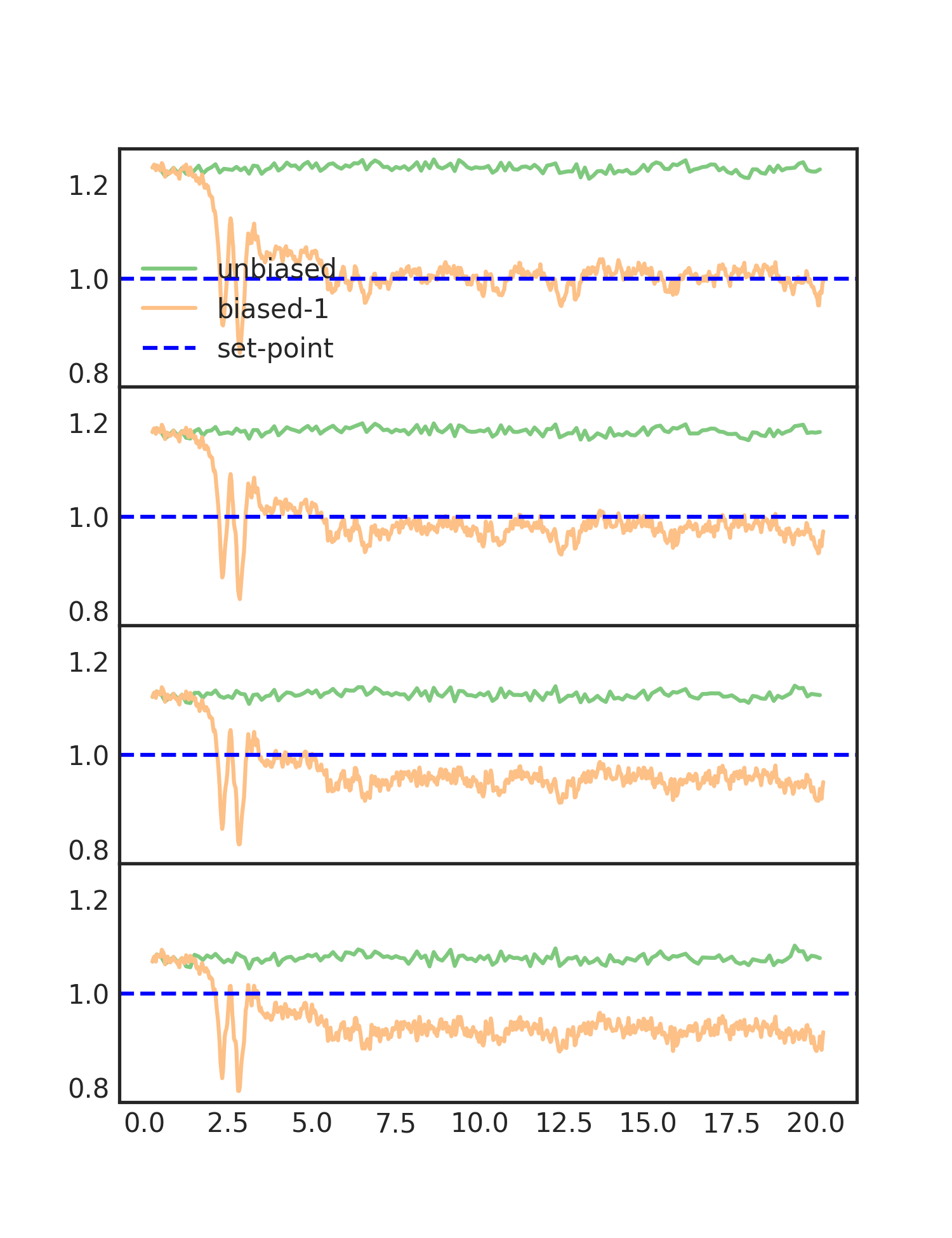
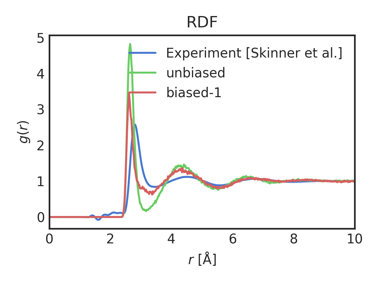
Each of the subplots is one of the coordination number moments. They are scaled to their set-points, so that the y-axes are similar. We can now see the effect of biasing more moments. The RDF after biasing with improvement is shown below
Changing the number of moments
Using the the same starting file, add another set-point
moments. Again, copy the biased.plumed file to make a
biased-2.plumed file with the EDS information. Now add another entry to the ARG on the eds: line.
The entry is cn1.mean, so that you’ll now have ARG=cn0.mean,cn1.mean. Run the simulation
and analyze the results
docker run --rm -it -v `pwd`:/home/whitelab/scratch whitelab/tutorial-lammps-cn lammps -var name biased-2 -in lammps.in
docker run --rm -it -v `pwd`:/home/whitelab/scratch whitelab/tutorial-lammps-cn python3 analyze_run.py unbiased biased-1 biased-2
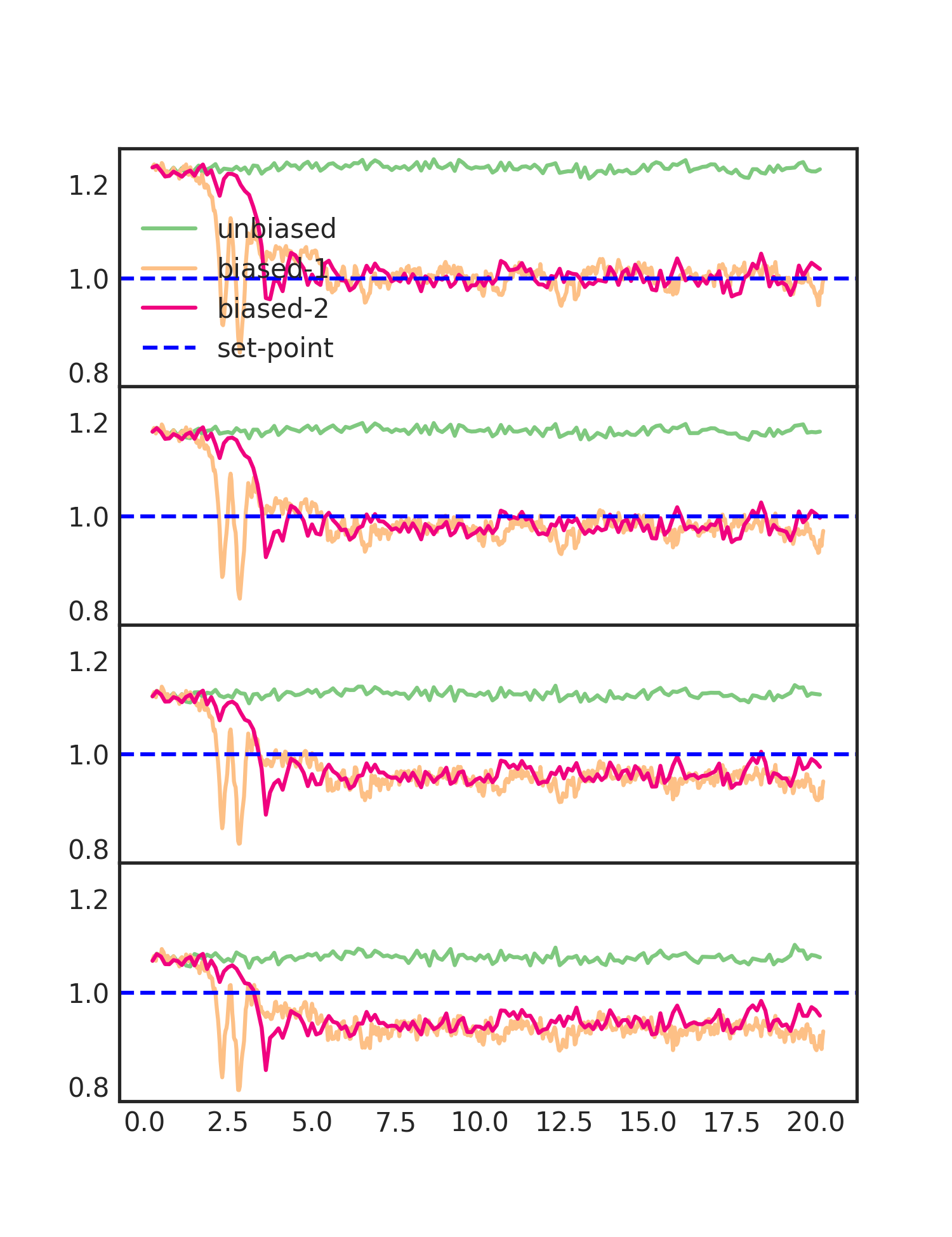
The additional moment provides, arguably, a little improvement but not as much as going from no bias to one moment. This is because the moments are correlated and there are diminishing returns to adding more bias. You can try adding more to see this effect (make sure to extend the simulation time).
You can get some insight into the algorithm from the diagnostic plot
(biases_comparison.png), which shows each the parameters used to
calculate the EDS updates. This plot is shown below for 1,2 and 4
moments.
Cleaning up
If you’d like to make the directory clean again to restart the
tutorial, run git clean -fX.
References
- White, A. D., Knight, C., Hocky, G. M., & Voth, G. A. (2017). Communication: Improved ab initio molecular dynamics by minimally biasing with experimental data. Journal of Chemical Physics, 146(4). https://doi.org/10.1063/1.4974837
- White, A., Dama, J., & Voth, G. A. (2015). Designing Free Energy Surfaces that Match Experimental Data with Metadynamics. Journal of Chemical Theory and Computation, 150430155138001. https://doi.org/10.1021/acs.jctc.5b00178
- Bonomi, M., Branduardi, D., Bussi, G., Camilloni, C., Provasi, D., Raiteri, P., Donadio, D., Marinelli, F., Pietrucci, F., Broglia, R. A., & Parrinello, M. (2009). PLUMED: A portable plugin for free-energy calculations with molecular dynamics. Computer Physics Communications, 180(10), 1961–1972. https://doi.org/10.1016/j.cpc.2009.05.011
- Skinner, L. B., Huang, C., Schlesinger, D., Pettersson, L. G. M., Nilsson, A., & Benmore, C. J. (2013). Benchmark oxygen-oxygen pair-distribution function of ambient water from x-ray diffraction measurements with a wide Q-range. The Journal of Chemical Physics, 138(7), 074506. https://doi.org/10.1063/1.4790861